
Marginal Revolution University
Published on 25 Apr 2017The long-run aggregate supply curve is actually pretty simple: it’s a vertical line showing an economy’s potential growth rates. Combining the long-run aggregate supply curve with the aggregate demand curve can help us understand business fluctuations.
For example, while the U.S. economy grows at about 3% per year on average, it does tend to fluctuate quite a bit. What causes these fluctuations? One cause is “real shocks” that affect the fundamental factors of production. Droughts, changes to the oil supply, hurricanes, wars, technological changes, etc. can all have big and potentially far-reaching consequences.
Next week, we’ll dig into why wages are considered “sticky,” or slow to change.
December 30, 2018
The Long-Run Aggregate Supply Curve
November 23, 2018
The Aggregate Demand Curve
Marginal Revolution University
Published on 18 Apr 2017This wk: Put your quantity theory of money knowledge to use in understanding the aggregate demand curve.
Next wk: Use your knowledge of the AD curve to dig into the long-run aggregate supply curve.
The aggregate demand-aggregate supply model, or AD-AS model, can help us understand business fluctuations. In this video, we’ll focus on the aggregate demand curve.
The aggregate demand curve shows us all of the possible combinations of inflation and real growth that are consistent with a specified rate of spending growth. The dynamic quantity theory of money (M + v = P + Y), which we covered in a previous video, can help us understand this concept.
We’ll walk you through an example by plotting inflation on the y-axis and real growth on the x-axis — helping us draw an aggregate demand curve!
Next week, we’ll combine our new knowledge on the AD curve with the long-run aggregate supply curve. Stay tuned!
November 21, 2018
Allied War Economy During World War 1 I THE GREAT WAR Special
The Great War
Published on 19 Nov 2018Check Out Supremacy 1914: https://www.supremacy1914.com/index.p…
Financing and supplying the First World War was a huge economic undertaking that influenced the British, French, American and Italian economies profoundly and shaped the global balance of power.
November 2, 2018
Intro to Business Fluctuations
Marginal Revolution University
Published on 11 Apr 2017This wk: Get acquainted with the basics of business fluctuations as we dive back into the final videos of our Macro course.
Next wk: Learn the basics of the aggregate demand-aggregate supply model.
Economic growth doesn’t happen at a steady pace; there are ebbs and flows. Prosperity on the national level depends on a country having good institutions in place. The factors of production – human capital, physical capital, and ideas – are also critical. And these variables often change, sometimes drastically.
In the United States, economic growth has averaged at about 3.2% for the past sixty years. But if you Google “US economic growth FRED,” you’ll quickly see that it’s not a smooth trend up. Instead, there are plenty of peaks and valleys, even though the U.S. has a relatively stable economy. Economists refer to these ups and downs around a country’s long-term GDP growth trend as “business fluctuations.”
“Recessions” are significant and widespread declines in employment and real income. But not only do people become unemployed during a recession, but capital and land often go un- or underused. This suggests that an economy is operating below its potential because resources are being wasted.
Recessions, large or small, are less than ideal states for an economy. We want people and resources well employed to produce more prosperity.
Over the next few videos, we’ll explore the basics of a model of business fluctuations called the aggregate demand-aggregate supply (AD-AS) model. We’ll put the model to use to look at how shocks affect an economy, and what policy can do to minimize the damage. Finally, we’ll apply the model to explain some of the largest economic catastrophes in United States’ history.
October 13, 2018
Why Governments Create Inflation
Marginal Revolution University
Published on 14 Feb 2017Inflation can carry with it quite a few costs. But some governments, like Zimbabwe under President Robert Mugabe in the early 2000s, will go out of their to way to create inflation. Why?
Well, in the Zimbabwe example, the government printed the money and used it to buy goods and services. The ensuing hyperinflation acted as a tax that transferred wealth from the citizens to the government.
However, this is a fairly uncommon reason. Inflation doesn’t make for a good tax and it’s a last resort for desperate governments that are otherwise unable to raise funds.
There are other benefits to inflation that would make governments want to create it. In the short run, inflation can actually boost economic output. However, as we’ve previously covered, an increase in the money supply leads to an equal increase in prices in the long run.
If there’s a recession, governments might create inflation to spur productivity and ease the economic downturn. However, this type of inflationary boosting can be abused. Long-term boosting causes people to simply expect and prepare for it.
Reducing inflation is also costly. If the process is reversed and the growth in the money supply decreases, we get disinflation. Unemployment will likely increase in the short run and an economy can go through a recession. But in the long run, prices will adjust as well.
Inflation can be a neat trick for governments to boost productivity in an economy. But it can easily get out of hand and has even been likened to a drug. Once you start, you need more and more. And stopping is awfully painful as the economy shrinks.
This concludes our section on Inflation and the Quantity Theory of Money. Up next in Principles of Macroeconomics, we’ll be digging into Business Fluctuations.
October 6, 2018
QotD: Macroeconomics
[I]t’s not too much to say that macroeconomics in the Samuelsonian-Keynesian mode abstracts away from most of what is essential in economics. Market processes and entrepreneurial searches for profit; specialization; the complementarity of different capital goods with each other and with labor; the role of relative prices; the reality and importance of institutions; the reality and importance of the fact that politicians are relatively uninformed and self-interested agents. These important aspects of economic and social reality are either ignored or treated haphazardly in too much of what is called “macroeconomics.”
Don Boudreaux, “Quotation of the Day…”, Café Hayek, 2016-11-05.
October 2, 2018
Costs of Inflation: Financial Intermediation Failure
Marginal Revolution University
Published on 7 Feb 2017In the previous video, we learned that inflation can add noise to price signals resulting in some costly mistakes from price confusion and money illusion. Now, we’ll look at how it can interfere with long-term contracting with financial intermediaries.
Let’s say you want to take out a big loan, such as a mortgage on a house. The financial intermediary (in this case, a commercial bank) is going to charge you an interest rate as their profit for loaning you the money. In this situation, inflation has the potential to work against you or it can work against the bank.
If the bank charges you a nominal interest rate (i.e., the interest rate on paper before taking inflation into account) of 5% and inflation climbs unexpectedly to 10% for the year, the real interest rate (nominal minus inflation) falls to -5%. The bank actually loses money. However, if inflation has been higher and banks are charging 15% for mortgages and inflation rates fall unexpectedly to 3%, you’re stuck paying a real interest rate of 12%!
The above scenarios are similar to what actually happened in the United States in the 1960s and 1970s. Inflation was low in the 60s. But then in 70s, inflation rates climbed up unexpectedly. People that purchased a home in the 60s lucked out with low interest rates on their mortgages coupled with higher inflation, and many were able to pay off the loans more quickly than expected. But anyone that purchased a higher interest rate mortgage in the 70s only saw inflation fall back down. It was good for the banks and a costly choice for the homeowners. They were saddled with a high-interest mortgage while lower inflation meant a lower increase in wages.
It’s not that the people buying homes in the 1960s were smarter than those in the 70s. As we’ve noted in previous videos, inflation can be very difficult to predict. When banks expect that inflation might be 10% in the coming years, they will generally adjust their nominal interest rates in order to achieve the desired real interest rate. This relationship between real and nominal interest rates and inflation is known as the Fisher effect, after economist Irving Fisher.
We can see the Fisher effect in the data for nominal interest rates on U.S. mortgages from the 1960s through today. As inflation rates rise, nominal interest rates try to keep up. And as the inflation rates fall, nominal interest rates trail behind.
Now, if inflation rates are both high and volatile, lending and borrowing gets scary for both sides. Long-term contracts like mortgages become more costly for everyone with much higher risk, so it happens less. This is damaging for an economy. Coordinating saving and investment is an important function of the market. If high and volatile inflation is making that inefficient and less common, total wealth declines.
Up next, we’ll explore why governments create inflation in the first place.
September 6, 2018
Costs of Inflation: Price Confusion and Money Illusion
Marginal Revolution University
Published on 2 Feb 2017The inflation rate can be somewhat volatile and unpredictable. For example, let’s take the period between 1964 and 1983 in the U.S. The inflation rate jumped around from 1.3% in 1964 to 5.9% in 1970, and all the way up to 14% in in 1980, before dipping back down to 3% in 1983. These dramatic changes, though still fairly mild in the realm of inflation, caught people off-guard.
Peru’s inflation rates in the late 1980s through the early 1990s were on even more of a rollercoaster. Clocking in at 77% in 1986, its inflation rate was already quite high. But by 1990, it had jumped to 7,500%, only to fall to 73% a mere two years later.
High and volatile inflation rates can wreak havoc on the price system where prices act as signals. If the price of oil rises, it signals scarcity of that product and allows consumers to search for alternatives. But with high and volatile inflation, there’s noise interfering with this price signal. Is oil really more scarce? Or are prices simply rising? This leads to price confusion – people are unsure of what to do and the price system is less effective at coordinating market activity.
Money illusion is another problem associated with inflation. You’ve likely experienced this yourself. Think of something that you’ve noticed has gotten more expensive over the course of your lifetime, such as a ticket to the movies. Is it really that going out the movies has become a pricier activity, or is it the result of inflation? It’s difficult for us to make all of the calculations to accurately compare rising costs. This is known as “money illusion” – or when we mistake a change in the nominal price with a change in the real price.
Inflation, especially when it’s high and volatile, can result in some costly problems for everyone. Next up, we’ll look at how it redistributes wealth and can break down financial intermediation.
August 20, 2018
Causes of Inflation
Marginal Revolution University
Published on 24 Jan 2017In the last video, we learned the quantity theory of money and its corresponding identity equation: M x V = P x Y
For a quick refresher:
•M is the money supply.
•V is the velocity of money.
•P is the price level.
•And Y is the real GDP.
In this video, we’re rewriting the equation slightly to divide both sides by Y and explore the causes behind inflation. What we discover is that a change in P has three possible causes – changes in M, V, or Y.
You probably know that prices can change a lot, even over a short period of time.
Y, or real GDP, tends to change rather slowly. Even a seemingly small jump or fall in Y, such as 10% in a year, would signal astonishing economic growth or a great depression. Y probably isn’t our usual culprit for inflation.
V, or the velocity of money, also tends to be rather stable for an economy. The average dollar in the United States has a velocity of about 7. That may fall or rise slightly, but not enough to influence prices.
That leaves us with M. Changes in the money supply are the driving factor behind inflation. Put simply, when more money chases the same amount of goods and services, prices must rise.
Can we put this theory to the test? Let’s look at some real-world examples and see if the quantity theory of money holds up.
In Peru in 1990, hyperinflation came into full swing. If we track the growth rate of the money supply to the growth rate of prices, we can see that they align almost perfectly on a graph with both clocking in around 6,000% that year.
If we plot the growth rates of the money supply along with the growth rates of prices for a many countries over a long stretch of time, we can see the same relationship.
We’ll wrap-up the causes of inflation with three principles to keep in mind as we continue exploring this topic:
•Money is neutral in the long run: a doubling of the money supply will eventually mean a doubling of the price level.
•“Inflation is always and everywhere a monetary phenomena.” – Milton Friedman
•Central banks have significant control over a nation’s money supply and inflation rate.
August 12, 2018
Misunderstanding what the trade deficit represents
In a post from last week, Tim Worstall explains why Donald Trump is wrong about the economic impact of a trade deficit:
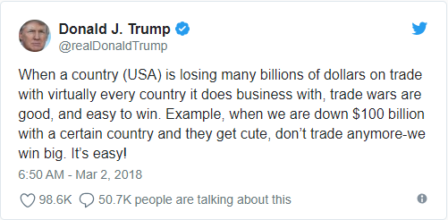
I should note here that I didn’t, because as a foreigner I can’t, support The Donald at the last election. But I didn’t support Hillary even more. So this is more about really, actually, insisting that Trump is wrong on trade issues rather than just the more general he’s wrong about everything common in the US press.
[…]
What Trump, DiMicco and Navarro are getting wrong is this, the GDP equation.
Y = C+I+G+(X-M)GDP is consumption plus investment plus government spending plus the trade balance – and minus it if there’s a trade deficit. So people look at this and think yep, if there’s a trade deficit than that makes Y, GDP, smaller!
But this is a mistake, an error. For, as the textbook immediately goes on to explain, what is it that we do with imports? Well, we either consume them, use them in investments or government buys them. So all imports are already in C and I and G. Meaning that if we don’t deduct them we’ll be double counting them. So, to avoid double counting we subtract them.
Trump and his advisers are simply wrong on this. The trade deficit doesn’t reduce the size of the economy. They’re getting it wrong simply because they’re not reading the second page of the explanation of the GDP equation.
August 9, 2018
Quantity Theory of Money
Marginal Revolution University
Published on 17 Jan 2017The quantity theory of money is an important tool for thinking about issues in macroeconomics.
The equation for the quantity theory of money is: M x V = P x Y
What do the variables represent?
M is fairly straightforward – it’s the money supply in an economy.
A typical dollar bill can go on a long journey during the course of a single year. It can be spent in exchange for goods and services numerous times. In the quantity theory of money, how many times an average dollar is exchanged is its velocity, or V.
The price level of goods and services in an economy is represented by P.
Finally, Y is all of the finished goods and services sold in an economy – aka real GDP. When you multiply P x Y, the result is nominal GDP.
Actually, when you multiply M x V (the money supply times the velocity of money), you also get nominal GDP. M x V is equal to P x Y by definition – it’s an identity equation.
You can think about the two sides of the equation like this: the left (M x V) covers the actions of consumers while the right (P x Y) covers the actions of producers. Since everything that is sold is bought by someone, these two sides will remain equal.
Up next, we’ll use the quantity theory of money to discuss the causes of inflation.
July 17, 2018
Measuring Inflation
Marginal Revolution University
Published on 10 Jan 2017Inflation is common in a modern economy. Shifts in supply and demand for goods and services cause prices to change accordingly. When the average level of prices rises, that’s inflation. It means that you’ll need more money to purchase the same stuff.
Inflation in the United States can be measured using the Bureau of Labor Statistics’ Consumer Price Index (CPI) – a weighted average of the price increases. We can calculate the inflation rate by the percentage change in the CPI over a given period of time.
How much do prices actually change? Well, using FRED, we can see that, over the past thirty-three years, prices have more than doubled. That may seem like a lot. However, wages have also risen, on average, by more than prices during that time period. Inflation doesn’t necessarily mean that we’re worse off.
The inflation rate in the United States has averaged at about 2.5% per year since 1980, which is fairly low and indicative of a stable economy. Prices may be increasing, but the changes are small. Wages have time to catch up. You can be confident that the $5 in your pocket isn’t going to be worth drastically less in a year.
Let’s take a look at a different scenario — one that’s playing in Venezuela right now. As the country faces an economic crisis, inflation is skyrocketing. Rates reached 180% in 2015 and have continued to rise since. 5 bolívar in your pocket could be worth less even by the end of the day.
But Venezuela still doesn’t compare to the hyperinflation that Zimbabwe experienced in the 2000s, reaching dizzying rates of billions of a percent per month. (See MRU’s previous video for more!)
While some inflation is perfectly normal, high rates of inflation make it difficult for consumers to use a nation’s currency. If the value is changing a lot by the week, day, or even minute, people don’t want to hold onto or accept the currency for goods and services — leading to a full blown currency crisis.
Up next, we’ll take a deeper dive into what causes inflation and its consequences.
July 7, 2018
Zimbabwe and Hyperinflation: Who Wants to Be a Trillionaire?
Marginal Revolution University
Published on 3 Jan 2017How would you like to pay $417.00 per sheet of toilet paper?
Sound crazy? It’s not as crazy as you may think. Here’s a story of how this happened in Zimbabwe.
Around 2000, Robert Mugabe, the President of Zimbabwe, was in need of cash to bribe his enemies and reward his allies. He had to be clever in his approach, given that Zimbabwe’s economy was doing lousy and his people were starving. Sow what did he do? He tapped the country’s printing presses and printed more money.
Clever, right?
Not so fast. The increase in money supply didn’t equate to an increase in productivity in the Zimbabwean economy, and there was little new investment to create new goods. So, in effect, you had more money chasing the same goods. In other words, you needed more dollars to buy the same stuff as before. Prices began to rise — drastically.
As prices rose, the government printed more money to buy the same goods as before. And the cycle continued. In fact, it got so out of hand that by 2006, prices were rising by over 1,000% per year!
Zimbabweans became millionaires, but a million dollars may have only been enough to buy you one chicken during the hyperinflation crisis.
It all came crashing down in 2008 when — given that the Zimbabwean dollar basically ceased to exist — Mugabe was forced to legalize transactions in foreign currencies.
Hyperinflation isn’t unique to Zimbabwe. It has occurred in other countries such as Yugoslavia, China, and Germany throughout history. In future videos, we’ll take a closer look at inflation and what causes it.
June 19, 2018
Women Working: What’s the Pill Got to Do With It?
Marginal Revolution University
Published on 29 Nov 2016At the turn of the century, it was rare for a woman to get a college degree or join, and stay in, the workforce. One trailblazer was Katherine McCormick. She was the second woman ever to graduate from MIT, a suffragist, advocate for women’s education, and later philanthropist. McCormick was also a staunch supporter of birth control, going so far as to smuggle contraceptives into the United States at a time when they were illegal or highly regulated.
In the 1950s, the birth control pill was extremely controversial. Funding for its development had been pulled. McCormick stepped in and, over time, contributed nearly $23 million (in today’s dollars) of her own money to research efforts. Her financial involvement was instrumental in achieving FDA approval and widespread acceptance of “the pill.”
But what does the the pill have to do with female education or women working? For the very first time, women were in control over if and when they would have children.
Since the mid-1960s, shortly after the pill was approved as a contraceptive in the United States, female education and labor force participation rates have skyrocketed. With the ability to control when they will have children, women are able to better plan for their academic and professional future. We may take it for granted today, but half a century ago, the pill changed the game for working women.
June 5, 2018
Taxing Work
Marginal Revolution University
Published on 22 Nov 2016For most people in developed countries, retirement comes down to a choice: weighing the costs and benefits of continuing to work vs. leisure. An important factor influencing an individual’s decision is their government’s tax and retirement policies.
Most developed countries offer a government-run retirement system with benefits that kick-in at a certain age. That age varies from country to country, usually starting when a worker reaches their early sixties.
Of course, not everyone wants to retire simply because they can receive benefits. People that really love their work may choose not to retire. In some countries, though, that decision can be heavily penalized through lost retirement benefits.
Taxes on earnings plus penalties, like losing retirement benefits, gives us an implicit tax rate. Countries with higher implicit tax rates for older workers see a much lower labor force participation rate for people considered retirement age.
As you might imagine, these government policies on retirement can be extremely costly. Many European governments that penalize non-retirement have been working to reform these policies and reduce implicit tax rates for elderly workers.
In the Netherlands, which had one of the highest implicit tax rates in the 1990s, an older worker could have actually had to pay to work. Since the Netherlands reformed their policies surrounding retirement, they’ve seen an increase in the labor force participation rate for older workers.
In the next video, we’ll cover another big influence on female labor force participation: The Pill.