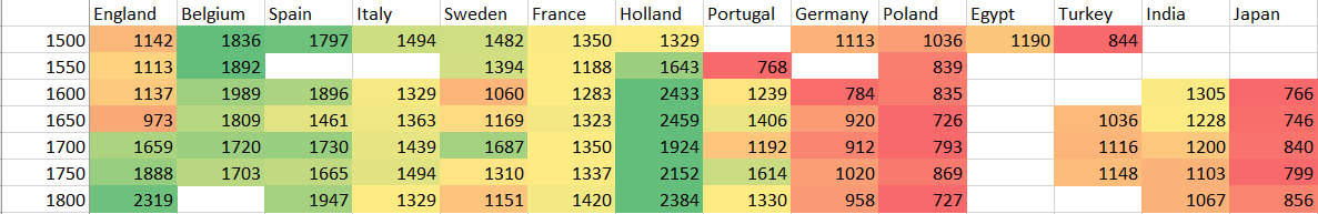
This post at Continental Telegraph a few days back reminded me I wanted to get around to gathering some of my older posts about the reasons to take the official GDP numbers from the Chinese government with more than just a pinch of salt. Here’s my very first rant on the topic from 10 August, 2004 (original expired URL – http://bolditalic.com/quotulatiousness_archive/000323.html):
On my way in to work this morning, I heard a stock advisor doing his best to make reasonable assumptions about what the average listener needed to know about the economy. This guy has been pretty level-headed in the past, but this morning’s talk just got my head ready to explode.
The topic of discussion was the Chinese economy and how the Chinese central bank was having to take greater efforts to rein in economic expansion. He talked about how many different sectors of the North American economy were, to greater or lesser degree, depending more and more on Chinese growth to increase their own investments and output. The idea that the Chinese economy was "overheating" was bandied about. He closed by indicating that a slight drop in the official growth rate from 9.8% to 9.6% showed that the Chinese central bank was seeing some results from their intervention in the economy.
There are so many things wrong here that I’m almost at a loss where to start. While there is no doubt that China is a fast-growing economy, the most common mistake among both investors and pundits is to assume that China is really just like South Carolina or Ireland … a formerly depressed area now achieving good results from modernization. The problem is that China is not just the next Atlanta or Slovenia. China is still, more or less, a command economy with a capitalist face. One of the biggest players in the Chinese economy is the army, and not just in the sense of being a big purchaser of capital goods (like the United States Army, for example).
The Chinese army owns or controls huge sectors of the economy, and runs them in the same way it would run a division or an army corps. The very term "command economy" would seem to have been minted to describe this situation. The numbers reported by these "companies" bear about the same resemblance to reality as those posted by Enron or Worldcom. With so much of their economy not subject to profit and loss, every figure from China must be viewed as nothing more than a guess (at best) or active disinformation.
Probably the only figures that can be depended upon for any remote accuracy would be the imports from other countries — as reported by the exporting firms, not by their importing counterparts — and the exports to other countries. All internal numbers are political, not economic. When a factory manager can be fired, he has his own financial future at stake. When he can be sentenced to 20 years of internal exile, he has his life at stake. There are few rewards for honesty in that sort of environment: and many inducements to go along with what you are told to do.
Under those circumstances, any growth figures are going to be aggregated from all sectors, most of which are under strong pressure to report the right numbers, not necessarily corresponding with any real measurement of economic activity. So, if the economic office wants to see a drop in the economy, that’s what they’ll get.
Basing your own personal financial plans on numbers like this would quickly have you living in a cardboard box under a highway overpass. Companies in the soi-disant free world have shareholders or owners to answer to. Companies in China exist in a totally different environment.
I returned to the same topic on October 25, 2004, triggered by yet another talking head on the radio under the heading “More Economic Voodoo — or is that Feng Shui?” (original URL – http://www.bolditalic.com/quotulatiousness_archive/000580.html):
Again this morning, I was listening to my local jazz radio station on the way in to work. As usual, they had a broker from CIBC Wood Gundy giving portfolio advice at about 9:20 a.m. Today’s talk was about investing in China, and how the markets have been reacting to the recent small drop in the official GDP growth figures released by the Chinese central bank.
This time, the emphasis was on the idea that in spite of the breathtaking growth figures, Chinese firms still are not particularly profitable and that therefore there are better ways of investing your money to benefit from all that growth. Unlike the last time I addressed this issue, this time I thought that the advisor was actually making pretty good sense. The incredible transformation of China from a pure command-driven economy to a mixed economy will certainly provide lots of opportunities for people to get rich; it will also provide even more opportunities to lose big money.
Much of the problem is that even now, the Chinese economy is not particularly free: the official and unofficial controls on the economy provide far too many opportunities for rent-seeking officialdom to play favourites and cripple antagonists (and for once, "cripple" is not just a bit of hyperbole). Any numbers provided by the Chinese authorities cannot be depended upon, and should probably only be viewed as an indication of what the Chinese government wants the outside world to believe.
Even in a relatively free economy like Canada, the underground economy can be huge, with plenty of economic activity happening out of reach of the taxman. In China, where everybody was raised in an environment where providing the "wrong" answer to your leader could get you imprisoned (or executed) as an economic criminal, the numbers upon which the bankers and financial officials depend can only be described as extremely unreliable.
Update 26 October: The Last Amazon asks a highly pertinent and pointed question:
In the past week, the Globe and Mail has been featuring the economic engine that China has become. Its economy is thriving so much so that Chinese government owned companies like China Minmetals Corp (which had revenues in 2003 of USD$11.7 billion) is currently negotiating to buy outright 100% of the stock of the Canadian mining corporation, Noranda Inc. The total stock is estimated at approximately CDN$6.7 billion.
If the Chinese government can afford to buy Noranda Inc. why hasn’t anyone asked when China will reimburse the overburdened Canadian taxpayers of this fair land for the Cdn$65.4 million that has been given to China as foreign aid?
I managed to stay away from the topic until April 13, 2007, when I posted “The Chinese Economy”, which largely quoted from my first two posts (old URL – http://bolditalic.netfirms.com/quotulatiousness_archive/003649.html):
Everyone must have heard many different variations on how incredible the Chinese economy is: spectacular growth, innovations galore, etc., etc. And there’s much truth to it — China has been industrializing at a mind-croggling pace. At least, the visual evidence says so. The economic data coming out of China is, to be kind, not as dependable as similar data from most other countries. […]
Three years on, I must retract a tiny bit there … Enron’s and Worldcom’s figures, while deliberately misleading, were refutable (and the culprits taken to court). […]
Samizdata links to a brief Tyler Cowen post which includes this quote:
…of the 3,220 Chinese citizens with a personal wealth of 100 million yuan ($13 million) or more, 2,932 are children of high-level cadres. Of the key positions in the five industrial sectors – finance, foreign trade, land development, large-scale engineering and securities – 85% to 90% are held by children of high-level cadres.
That’s even higher than I expected. But it’s an excellent example of what I originally wrote about back in 2004: the economy isn’t free, and the beneficiaries are disproportionally those who are politically well-connected. Caveat investor.
And that was when I discovered that my “full” backup of files from the old site is actually missing nearly a year of posts from May 2008 to May 2009 (when I moved to the current site). I vaguely recall that Jon (my former virtual landlord) was having problems with limited storage on that site — I was just a freeloading guest — so perhaps one of the things we lost was the auto-archiving after we reached a certain capacity.
Thanks to the Wayback Machine, I found a couple of other entries but they were often just rehashes of the first two posts interspersed with quotations from articles I felt were being too Pollyanna-ish about the Chinese economic numbers, like this one from May 2, 2008:
Those untrustworthy Chinese economic numbers
Regular readers will know that I’ve been a long-term skeptic about the economic figures reported by the Chinese government (for example, here and here back in 2004). As a result, this post at the Economist is not very surprising:
As China’s importance in the global economy increases, investors are paying more attention to its economic numbers. Yet the country’s official statistics are notoriously ropy. Some commentators accuse China’s government of overstating GDP growth for political reasons, others complain that the official inflation rate is fraudulently low. So which data can you trust?
One reason to be suspicious of GDP figures is that China is always one of the first countries to report them, usually only two weeks after the end of each quarter. Most developed economies take between four and six weeks to produce them.
However, The Economist still feels that the Chinese economy is larger than reported. My sense of distrust in the figures argues for it being neither as big nor as robust as the reported figures indicate. They’re professional economic reporters … I’m a guy typing a blog entry. I wonder what the long-term odds are for either of us to be closer to the truth?
It’s tough to disagree with this, though:
The prize for the dodgiest figures goes to the labour market. The quarterly urban unemployment rate is meaningless because it excludes workers laid off by state-owned firms as well as large numbers of migrant workers, who normally live in urban areas but are not registered. Wage figures are also lousy. There has recently been much concern about the faster pace of increase in average urban earnings. But this series does not cover private firms, which are where most jobs have been created in recent years.
Now that China is such an engine of global growth, it urgently needs to improve its economic data. Only a madman would drive a juggernaut at full speed with a faulty speedometer, a cracked rear-view mirror and a misty windscreen.
By this point, Jon was referring to my obsession with bogus Chinese economic statistics as my “hobby horse” … yet it wasn’t unknown for him to send me links to articles on that very topic. Here’s another post, courtesy of the Wayback Machine, from January 23, 2009:
China’s economic situation
There’s an article at The Economist today that shows a touching belief in the magic of the Chinese economy. The reported Gross Domestic Product has fallen to “only” 5.8%. The Economist‘s writer spends much of the article worrying about this gloomy report:
New figures show that China’s GDP growth fell to 6.8% in the year to the fourth quarter, down from 9% in the third quarter and half its 13% pace in 2007. Growth of 6.8% may still sound pretty robust, but it implies that growth was virtually zero on a seasonally adjusted basis in the fourth quarter.
Industrial production has slowed even more sharply, growing by only 5.7% in the 12 months to December, compared with an 18% pace in late 2007. Thousands of factories have closed and millions of migrant workers have already lost their jobs. But there could be worse to come. Chinese exports are likely to drop further in coming months as world demand shrinks. Qu Hongbin, an economist at HSBC, forecasts that exports in the first quarter could be 19% lower than a year ago. 2009 may well see the first full-year decline in exports in more than a quarter of a century.
Economists have become gloomier about China’s prospects, with many now predicting GDP growth of only 5-6% in 2009, the lowest for almost two decades.
I’ve blogged about the Chinese economy on a few occasions (most recently here), generally with the same concern: that the numbers reported cannot be relied upon. The same is true here. Interestingly, the Economist article I linked to back in May makes this point quite well, yet today’s article appears to treat the Chinese government’s numbers as solid.
China has changed substantially from twenty years ago, and in many ways for the better. Most ordinary Chinese today are more free — economically anyway — than they were a generation ago, and there is a lot more opportunity for individuals to set up businesses and to succeed without needing Party connections. All this is indisputable … yet vast swathes of the Chinese economy are a legacy of the worst command-and-control period. It’s not an exaggeration to say that we can expect to discover the “official numbers” have absolutely no relationship to reality, because the numbers are compiled from various sources including both free-r quasi-capitalist companies and tottering government-owned (and often People’s Liberation Army-owned) conglomerates which cannot be depended upon to report anything accurately.
An example from this article: “a fall in electricity output of 6% in the year to the fourth quarter, down from average annual growth of 15% over the previous five years.” That’s not just a reduction in the rate of growth, that’s a reported drop in output of 6%. Imagine what the state of a European or Japanese/Korean economy running at only 94% of electricity … it’d be something you’d only see at times of severe economic contraction, not as a sign of a slow-down in growth.
Finally, on May 22, 2009, a final post on the topic at the old blog:
Official Chinese statistics
If you’ve read the blog for a while, you’ll know that I’m pretty skeptical about how believable the official statistics coming from the Chinese government may be. The Economist is somewhat undecided on the matter … sometimes publishing articles that treat the official numbers as legitimate and other times, showing more doubt:
Part of the recent optimism in world markets rests on the belief that China’s fiscal-stimulus package is boosting its economy and that GDP growth could come close to the government’s target of 8% this year. Some economists, however, suspect that the figures overstate the economy’s true growth rate and that Beijing would report 8% regardless of the truth. Is China cheating?
Economists have long doubted the credibility of Chinese data and it is widely accepted that GDP growth was overstated during the previous two downturns. In 1998-99, during the Asian financial crisis, China’s GDP grew by an average of 7.7%, according to official figures. However, using alternative measures of activity, such as energy production, air travel and imports, Thomas Rawski of the University of Pittsburgh calculated that the growth rate was at best 2%. Other economists reckon that Mr Rawski was too pessimistic. Arthur Kroeber of Dragonomics, a research firm in Beijing, estimates GDP growth was around 5% in 1998-99, for example. The top chart, plotting the official growth rate against estimates by Dragonomics, clearly suggests that some massaging of the government statistics may have gone on. The biggest adjustment seems to have been made in 1989, the year of political protests in Tiananmen Square. Officially, GDP grew by over 4%; Dragonomics reckons it actually declined by 1.5%.
Of course, The Economist doesn’t want to lose sales in China, so the last paragraph of the article blithely re-assures readers that things are improving and that the official numbers are much harder to fudge now than they used to be. That may well be true (I rather hope it is), but in the same way that you can get much more impressive growth from a very small base, you can become much more honest with your numbers when you’re starting from pure fiction.
[…] Let’s just say that I’m still unconvinced.
After that, my hobby-horse rides can be found by searching for “china economy” (or just click this link) on the current blog, or you can just peruse the China category.